Neural Networks
Internal
Overview
A neural network consists of several layers of activation units ("individual units" or "individual neurons"), where the output of one unit is connected to the inputs of all units of the successive layer. The behavior of an individual activation unit is described in the "Individual Unit" section. A neural network's topology, along with conventions and notations - which are essential to understand if you want to follow the linear algebra equations - are discussed in the "Topology" section.
A neural network produces predictions by forward propagating input, then activations, across its layers from left to right, until the output layer computes the hypothesis function, for a specific input sample. A single activation unit has a function similar to logistic regression, but instead of applying the logistic function only to a set of input features, it is applied successively to the input features and to activation values of intermediate layers. The intuition behind this behavior is that a neural network gets to learn its own internal features, often across several layers, instead of being constrained to process the input features and immediately produce a result. Practice shows that the network may learn interesting and complex features, which can lead to a better hypothesis.
The forward propagation process is described in detail in the "Forward Propagation" section.
Forward propagation computations are performed based on a set of parameters (or weights) that are obtained by training the network. Training the network, or "fitting the parameters", is performed by a backpropagation algorithm, which is described in the "Backpropagation" section.
Individual Unit
Individual neural network units are computational units that read input features, represented as an unidimensional vector x1 ... xn in the diagram below, and calculate the hypothesis function as output of the unit. The result of the hypothesis function is also called the "activation" of the unit.

Input Feature
In context of an individual processing unit, the input feature refers to an individual value fed to a single input of the unit. For units in the first layer, the features are individual elements of the input matrix, while for units in the hidden layers or the output layers, the features are the activation values of the computational units from the previous layer.
The input features are grouped into an input vector.
In most cases, an additional constant value x0=1 is added to the feature vector. x0 is not part of the feature vector, but it represents a bias value for the unit. In a multi-layer neural network, the bias values are provided by bias units.
Activation
The output value of the hypothesis function is also called the "activation" of the unit and it is conventionally named ai(j), where j is the layer the unit belongs to, and i is the index of the unit in the layer. For more details on notation, see Topology section below. The activation value is calculated by applying the logistic function to a linear combination of input features and parameters, thus the unit is referred to as a logistic unit with a sigmoid (logistic) activation function.
Parameters
Parameters are real values that are applied to the input vector as a linear combination. For neural networks, they are also known as weights. Conventionally, they are named θ (theta), and for a multi-layer neural network, the model parameters are collected in matrices named Θ. The naming convention is described in detail in the Topology section.
Topology

The total number of layers in the network is conventionally named L. Layer 1 is the input layer, layers 2, 3, ... L - 1 are the hidden layers, and layer L is the output layer.
The number of units in the layer l is conventionally named sl. This number does not include the bias unit, so the total number of units in a layer, including the bias unit, is sl + 1.
The total number of classes the network classifies, which is equal to the number of output units, is conventionally named K.
Activation ai(j) represents the activation of unit i in layer j. The input values x can be thought of as the activations of the input layer, conventionally named layer 1, and so they can be consistently named a1(1), a2(1), ... an(1). The input bias unit is a0(1)=1.
Θ(j) represents the matrix of parameters (weights) that controls function mapping from layer j to layer j + 1. Details on how these parameters are used in computing activation values are available in the Forward Propagation section.
Input Layer
The input layer, conventionally named "layer 1", consists of input nodes. The input layer provides the training values during the training phase, and the input values during the classification phase. A training set contains a number of samples (m), and each sample has a number of features (n). The training set is conventionally represented as a matrix X.

Output Layer
For multi-class classification, each y value of the training set is represented as a vector containing binary values. When an element of a specific class is matched, the corresponding unit in the output layer will product an "1" activation value, while all other units produce "0" activation values. The output layer has as many units as classes we are attempting to classify.

Forward Propagation
Forward propagation consists in calculating hΘ(x(i)) for any x(i) of the input set. This is done by assigning input (x(i)) to to layer 1, and then steping from left to right through layers, calculating linear combinations of inputs and parameters for a layer, conventionally named zi(j), and applying sigmoid function to them. The result of the sigmoid function provided unit activation values.

If the layer j has p units, not counting the bias unit, and layer j + 1 has q units, not counting the bias unit, then the parameter matrix Θ(j) controlling function mapping from layer j to layer j + 1 has q x (p + 1) elements. The "+1" comes from the addition of the bias node in layer j.
To compute the activation values of a layer j + 1, we calculate the weighted linear combination of the input values (or the activation values of the previous layer) zi(j + 1):

The vectorized implementation of forward propagation from layer j to layer j + 1 is averrable below:

To obtain the activation values of the output layer, we don't need to add the bias unit to the result vector.
Neural Network Training
The neural network training process has the objective of minimizing the network's cost function: given the cost function J(Θ), we want to find parameters Θ that minimize J(Θ). The network with the minimal cost function produces the best predictions. A minimization algorithm can minimize the cost function if we provide an implementation that can calculate J(Θ), given an arbitrary parameter matrix Θ input, and partial derivatives of J(Θ) over Θ. The process of training the network consists of:
1. Providing a regularized cost function. The regularized cost function for a neural network is described in the "Regularized Cost Function" section.
2. Providing the partial derivatives of J(Θ) over Θ. The numerical values for these partial derivatives are produced by the backpropagation algorithm, described in the "Backpropagation" section.
3. Executing the minimization algorithm.
Regularized Cost Function
The cost function for a multi-class neural network is a generalization of the logistic regression regularized cost function, as follows:

where the double sum adds the logistic regression regularized cost function over each of the K output units, and then adds the result over the entire length of the training set. In this expression, (hΘ(x))k represents the kth element of the output vector.
The regularization term sums all the squared values of all Θ matrices, except the terms corresponding to the bias values. The i index in this sum does not refer to the index of the row in the training set. Note that the regularization term is sometimes computing using the following formula, which yields the same result:

The MATLAB function that computes the regularization term for an individual Θ matrix:
function rt = regularizationTerm(lambda, m, Theta)

% We expect that the weights corresponding to the bias values
% are provided on the first column of the Theta matrix, so we
% drop them

if lambda == 0
    rt = 0;
else
    columns = size(Theta, 2);
    T = Theta(:, 2: columns);
    rt = (lambda / (2 * m)) * sum(sum(T .^ 2));
end
end
Backpropagation
The backpropagation algorithm computes the partial derivatives of the cost function J(Θ) over Θjk(l).
It does that by forward propagating a training set sample though the network, as described in the Forward Propagation section, until it obtains the hypothesis function values for the current matrix of parameters. At that point, the algorithm reverses course, and it starts to compare the hypothesis function values with the actual values y(i) provided by the training set, and then backwards, calculating weighted averages of the error terms of the nodes in the preceding (right) layer . This results in an "error term" δi(j) for each one that measures how much each node is responsible for any errors in the output. The algorithm uses this numerical value to:
1. Calculate the partial derivatives for the layer and accumulate them in a partial derivative matrix.
2. Backpropagate the errors to the previous layer, from right to left, and repeat the process. This part of the process is mathematically similar to forward propagation, except that the computations are flowing from the left to the right of the network.
This sequence is repeated in a loop for each sample of the training set.
Details for each stage are provided below:
Weight Initialization
Weights should be initialized randomly to avoid the problem of symmetric ways.
Forward Propagation
Described in the Forward Propagation above. At the end of forward propagation for a sample, the algorithm obtains the hypothesis function values for the current matrix of parameters Θ.
Compute Error Terms
This process starts with the output layer, where the error term is the difference between our network's results and the actual values coming from the training set, calculated with the following formula:
For inner layers, the error term δi(j) representing the "error" in the activation value ai(j) of the node i in layer j is calculated multiplying the transposed Θ(j) [p + 1 x q] for the layer with the vector [q x 1] containing error term values of the j + 1 layer to its right, then dropping the bias element from the resulted [p + 1 x 1] vector, and then doing element-wise multiplication with the derivative of the activation function g() evaluated with the input values given by z(j), which is a [p x 1] vector.
The above formula is true because it can be demonstrated that:

Calculate Partial Derivatives
Once the error terms for a layer are computed, and before propagating the errors to the previous layer, accumulate partial derivative values for this sample in Δ(j) for the layer.

Mathematically, each element of the error matrix Δ that controls error backpropagation between layer j and j + 1 is calculated as follows:
![]()
The errors accumulate with iterations over the training set as follows:
![]()
The corresponding vectorized expression is:

The partial derivative of the cost function J(Θ) over the elements of the Θ matrix is given by the formula:

where:
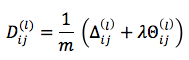 if j is not 0.
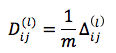 if j is 0.


MATLAB Code that Calculates Cost Function and Partial Derivatives
m = size(X, 1);

%Theta1 (hidden_layer_size, input_layer_size + 1)
%Theta2 (num_labels, hidden_layer_size + 1)

Delta1 = zeros(hidden_layer_size, input_layer_size + 1);
Delta2 = zeros(num_labels, hidden_layer_size + 1);

D1 = zeros(size(Delta1));
D2 = zeros(size(Delta2));
J = 0;

for i = 1:m

    % Assign inputs including the bias unit to the first layer of the network
    a1 = X(i, :)';
    a1biased = [1; a1];

    % Calculate z(2)
    z2 = Theta1 * a1biased;

    % Calculate a(2)
    a2 = sigmoid(z2);
    a2biased = [1; a2];

    % Calculate z(3)
    z3 = Theta2 * a2biased;

    % Calculate a(3)
    a3 = sigmoid(z3);

    % Cost vector over all output units
    yb = mapScalarToBinaryVector(num_labels, y(i));

    c = yb .* log(a3) + (1 - yb) .* log(1 - a3);

    % Cost scalar
    J = J + sum(c);

    % Calculate delta(3)

    d3 = a3 - yb;

    % Accumulate the partial derivative for this sample

    Delta2 = Delta2 + d3 * a2biased';

    % propagate the error backwards to layer 2

    d2biased = Theta2' * d3;

    % drop the error term corresponding to the bias unit

    d2 = d2biased(2:end);
    d2 = d2 .* sigmoidGradient(z2);

    % Accumulate the partial derivative for this sample

    Delta1 = Delta1 + d2 * a1biased';

end

J = (-1 / m) * J + regularizationTerm(lambda, m, Theta1) + regularizationTerm(lambda, m, Theta2);

D1 = Delta1 / m;
D2 = Delta2 / m;

% regularization
D1regTerm = (lambda / m) * [zeros(size(Theta1, 1), 1), Theta1(:, 2:size(Theta1, 2))];
D2regTerm = (lambda / m) * [zeros(size(Theta2, 1), 1), Theta2(:, 2:size(Theta2, 2))];

D1 = D1 + D1regTerm;
D2 = D2 + D2regTerm;