Algorithm Complexity

External

• https://en.wikipedia.org/wiki/Big_O_notation
• http://infotechgems.blogspot.com/2011/11/java-collections-performance-time.html

Internal

• Data Structures and Algorithms

Overview

Algorithm analysis is useful to determine the amount of resources consumed by an algorithm while solving a computational problem, as a function of its input size. In most cases the resource being consumed is running time. An analysis can also determine the requirements for memory, also referred to as space complexity, network bandwidth and other resources.

The concept of input size depends on the problem being addressed. In case of sorting algorithms, the most natural measure of input size is the number of items in the input. For the problem of multiplying two integers, the best measure of input size is the total number of bits needed to represent the input in binary notation. In the case of graph algorithms, there are two numbers that describe the input size: the graph's number of vertices and edges. If the problem involves two vectors whose size is unrelated, then the input size is also two-dimensional and consists of the lengths of both vectors.

The running time, or computational time of an algorithm on a particular input is usually very well predicted by the number of random-access machine primitive operations, or steps, executed.

Random-Access Machine (RAM)

An algorithm is usually analyzed in the context of a random-access machine (RAM), which is a theoretical model for the computing resources typically used by algorithms. A random-access machine has only one processor. In this model, instructions are executed one after another, with no concurrent operations, though extensions of the model exist for the case where we need to analyze multithreaded algorithms. Algorithms are implemented as computer programs for such a machine. The random-access machine mimics how real computers are designed, so it has instructions commonly found in real computers: arithmetic (add, subtract, multiply, divide, remainder, floor, ceiling), data movement (load, store, copy) and control (conditional branch, subroutine call and return). It is important to emphasize that each type of instruction takes a constant amount of time - this assumption is essential in algorithm analysis. This time is marked as c_i when analyzing a specific algorithm.

In accordance with how real computers are implemented, operations as multiplication with 2^k are also considered constant-time, because they are implemented by shifting left a number representation for k times, as long as k is no more than the number of bits in a computer word. Also, a statement calling a subroutine takes a constant amount of time, although the execution of the subroutine will usually not.

The data types in the RAM model are integer and floating point. The model assumes a limit on the size of each word of data: if the word size could grow arbitrarily, we could store large amounts of data in one word and operate on it in constant time, which is an unrealistic scenario.

A random-access machine does not attempt to model a memory hierarchy (caches or virtual memory). In some cases, memory hierarchy's effect is significant, but usually, RAM-model analyses are good predictors of performance on actual machines.

Time Complexity Analysis Method

We start by expressing the algorithm in random-access machine instructions. As mentioned above, each type of instruction takes a constant time c_i to execute, referred to as the cost of the instruction.

The running time of the algorithm is the sum of running times for each statement executed. A statement with a cost c_i that executes n times will contribute c_i⋅n to the total running time. When adding various costs, the terms of the same order can be coalesced: c₁n + c₂n + ... c_kn can be expressed as c⋅n.

Some statements may execute or not depending on which input of size n is given. From this perspective, an input may be the worst, leading to the longest running time, the best, leading to the shortest running time, or average. Additional complications in calculating the running time arise when we deal with recursive algorithms. Those aspects will be discussed below in the Recursive Algorithms and Recurrences section.

Worst-case Running Time

Time complexity analysis focuses on worst-case running time. The worst-case running time is the longest running time for any input of size n. The worst-case running time is important because it gives us an upper bound for the running time for any input, and knowing it provides a guarantee that the algorithm cannot do any worse. For some algorithms, the worst case occurs fairly often: for example, searching in a database when the information is not present. Also, the average case is often roughly as bad as the worst case. As we will see below, the O-notation provides a way to express asymptotic upper bounds to functions, so it is used when talking about running time for any situation, including worst-case running time.

Best-case Running Time

The best-case running time for an algorithm is the running time when the input is arranged in the best possible way, so the algorithm has to perform the minimal number of steps to solve the problem. An example is an already sorted array for insertion sort. As we will see below, we use the Ω-notation to describe the best-case running time of an algorithm.

Average-case Running Time

The average-case running time is the running time of an algorithm, in average, for a large number of different inputs. The average-case running time can be determined using probabilistic analysis.

More explanations on the difference between average-case running time and expected running time.

Expected Running Time

In general we expect that all inputs of a given size are equally likely, but in practice this may not be the case. In such situations we can use a randomized algorithm to allow probabilistic analysis and yield an expected running time.

Order of Growth of an Algorithm's Running Time

The result of the time complexity analysis method described above is a mathematical function of the input size.

A very common case, but by all means not the only case, is that the running time can approximated by a polynomial function in n, such as, for example a⋅n² + b⋅n + c. In this situation, we can consider only the highest-order term of the formula: a⋅n². We can also ignore the leading term's constant coefficient, since the constant factors are less significant than the other factor of the term in determining computational efficiency for large inputs.

The rate of growth or the order of growth of the algorithm's running time is the highest-order term, without coefficient. In this case of our example, the rate of growth is n².

One algorithm is considered to be more efficient than another if its worst-case running time has a lower order of growth, so that is why when we are analyzing the function describing the running time, we are usually interested in its order of growth.

Due to constant factors and lower-order terms, an algorithm whose running time has a higher order of growth might take less time for small inputs than an algorithm whose running time has a lower order of growth. However, for large enough inputs, the algorithm with lower order of growth will aways run faster. For example, comparing running time for two algorithms of which one is c₁n² and the other is c₂ n lg n, even if c₂ > c₁, no matter how much smaller c₁ is than c₂, there will always be a crossover point beyond which the c₂n lg n algorithm is faster.

Asymptotic Notation

When we look at input sizes large enough to make only the order of growth of an algorithm relevant, we say that we are analyzing the asymptotic efficiency of the algorithm.

Asymptotic efficiency is concerned with how the running time of the algorithm increases with the size input in the limit, as the size of the input increases without bound. Usually, an algorithm that is asymptotically more efficient is the best choice, for all but very small inputs.

To make easier to reason about asymptotic efficiency of various function expressing algorithms' running times, we can use the asymptotic notation. Asymptotic notation essentially designates classes, or sets of functions that behave asymptotically in the same way as the function used in the notation. Adding two function with the same asymptotic notation results in a function with the same asymptotic notation, and so on, and this simplifies reasoning when we estimate the algorithm's efficiency. While we mostly use the notation to describe algorithms running times, it actually applies to functions whose domain is the set of natural numbers. We can use asymptotic notation to function that describe space complexity, or to functions that have nothing to do with algorithms.

The notation abstracts away some details of the actual function: the lower-order terms of an asymptotically positive function can be ignored when determining the asymptotical bounds, because they are insignificant for large n. The terms of the same order can be coalesced. The coefficient (constant) of the highest-order term can be dropped, since it only changes the constants c₁ and c₂ in the definitions presented below by just a constant factor. All these can be done while the essence of the function - its asymptotic efficiency - is preserved.

Technically, a function f(n) belongs to a set such as O(g(n)) or Θ(g(n)), so it should be written as f(n) ∈ O(g(n)), but we conventionally write "f(n) = O(g(n))". For more details, see Using Asymptotic Notation in Equations and Inequalities.

Any constant function can be expressed as Θ(1). This notation is a minor abuse, because it does not indicate what variable is tending to infinity, but is accepted by convention.

Θ-notation

For a given function g(n), we denote by Θ(g(n)) the set of functions f(n) as follows:

Θ(g(n)) = {all f(n) : there exist positive constants c₁, c₂ and a integer n₀ such that 0 ≤ c₁g(n) ≤ f(n) ≤ c₂g(n) for all n ≥ n₀}

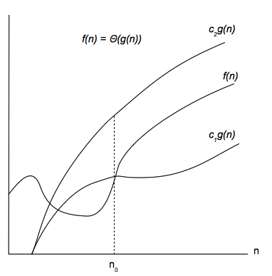
A function f(n) belongs to the set Θ(g(n)) if there exist positive constants c₁ and c₂ so f(n) is bounded by c₁g(n) and c₂g(n) for sufficiently large n. In other words, for all n ≥ n₀, function f(n) is equal to g(n) within a constant factor. We also say that g(n) is an asymptotically tight bound for f(n).

Θ-notation is a stronger notion that O-notation and Ω-notation, described below. That means f(n) = Θ(g(n)) implies f(n) = O(g(n)) and f(n) = Ω(g(n)).

For all values of n at and to the right of n₀, the value of f(n) lies at or above c₁g(n) and at or below c₂g(n).

O-notation

Unlike the Θ notation, the O notation is used to express an asymptotic upper bound. For a given function g(n), we denote by O(g(n)) the set of functions f(n) as follows:

O(g(n)) = {all f(n) : there exist a positive constant c and a integer n₀ such that 0 ≤ f(n) ≤ c⋅g(n) for all n ≥ n₀}

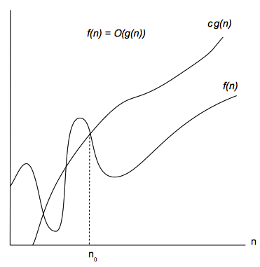
For all n ≥ n₀, function g(n) provides an upper bound to function f(n) within a constant factor.

Since O-notation provides an upper bound, if we use it to describe worst-case running time, then it characterizes the running time for any input. Worst-case running time is the running time we're most interested in, as argued above, and that is the reason the O-notation is most commonly used.

For all values n at and to the right of n₀, the value of the function f(n) is on or below c⋅g(n).

Ω-notation

The Ω notation is used to express an asymptotic lower bound. For a given function g(n), we denote by Ω(g(n)) the set of functions f(n) as follows:

Ω(g(n)) = {all f(n) : there exist a positive constant c and a integer n₀ such that 0 ≤ c⋅g(n) ≤ f(n) for all n ≥ n₀}

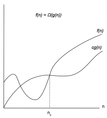
In other words, for all n ≥ n₀, function g(n) provides a lower bound to function f(n) within a constant factor. Informally, we say that under any circumstance, the algorithm cannot do better that. The Ω is used to describe the best-case running time of an algorithm.

For all values n at and to the right of n0, the value of the function f(n) is on or above c⋅g(n).

Using Asymptotic Notation in Equations and Inequalities

Technically, a function f(n) belongs to a set such as O(g(n)), Θ(g(n)) or Ω(g(n)), so it should be written as f(n) ∈ O(g(n)), but we conventionally write "f(n) = O(g(n))".

When the asymptotic notation stands alone on the right-hand side of an equation, as in the above example, or inequality, the equal sign means set membership. Example: f(n) = O(n²) means f(n) ∈ O(n²).

When the asymptotic notation appears in a formula, it is a stand-in for some anonymous function. The main reason to use the notation this way is to eliminate inessential details in an expression.

Because transitivity, reflexivity and symmetry apply to asymptotic notation, we can draw an analogy between the asymptotic comparison of two functions f() and g()( and the comparison of two real numbers:

• f(n) = O(g(n)) is like a ≤ b
• f(n) = Θ(g(n)) is like a = b
• f(n) = Ω(g(n)) is like a ≥ b

Recursive Algoritms and Recurrences

The running time of recursive algorithms can be analyzed using recurrences.

A recurrence, or a recurrence equation, is an equation or an inequality that describe the run time of a recursive algorithm for a problem of size n in terms of the running time on smaller inputs. Once the run time is expressed this way, we can use mathematical tools or other methods to solve the recurrence, which means obtaining asymptotic bounds on the run time of the algorithm.

Solving Recurrences

There are at least three method to solve recurrences:

Substitution Method

The method consists in guessing a bound and then using mathematical induction on the recurrence to prove the solution correct. We can guess a solution using a recursion tree. Examples on how to use mathematical induction to prove the bound is correct are available in CLRS page 83.

Recursion-Tree Method

The method consists in converting the recurrence into graphical tree representation whose nodes represent costs incurred at various level of the recursion. After we lay out the tree, we sum the costs within each level of the tree to obtain a set of per-level costs, then we sum all the per-level costs to determine the total cost of the recursion. The bound such guessed can be proven with the substitution method. Examples on how to build recursion trees are available in CLRS page 37 and page 88.

The Master Theorem

The master method is a method of analyzing running time of recursive algorithms by using the "master theorem". The master theorem applies to algorithms whose running times can be expressed as a recurrence equation. A generic form of a recurrence equation is:

T(n) = a⋅T(n/b) + f(n)

where a ≥ 1, b > 1 and f(n) is a function that approximates the non-recursive cost. Note that the above expression does include a boundary condition for n = 1. The reasons is that T(1) does not significantly change the solution to the recurrence, it may change it with a constant factor, but the order of growth will stay unchanged.

TODO CLRS page 93.

Analyzing Divide-and-Conquer Algorithms

For divide-and-conquer recursive problems, where solving the problem involves dividing the problem into a subproblems of size n/b of the original', applying the algorithm recursively a times on n/b-size problems and then combining the result, the run time can be expressed by the generic recurrence presented below. If the problem size is small enough (n ≤ c) the straightforward solution takes constant time, which is expressed as a constant function Θ(1).

       | Θ(1)                     if n ≤ c
T(n) = |
       | aT(n/b) + D(n) + C(n)    otherwise

where the D(n) is the cost of dividing the n-size problem into a subproblems, and the C(n) is the cost of combining the results.

Examples of Time Complexity Analysis

• Insertion sort
• Merge sort