Graph Search

Internal

• Graphs

Overview

Searching a graph is a fundamental problem in computer science. To search a graph means to systematically follow the edges of a graph and visit all the vertices of that graph. Techniques for searching a graph lie at the heart of the field of graph algorithms. There are many methods to search graphs, and the most known and used are breadth-first search and depth-first search.

Both breadth-first search and depth-first search algorithms are very efficient, in that they walk the entire graph in linear time of the number of vertices and edges O(n + m). A key implementation idea is to mark the nodes that have been visited already so the algorithm does not look at them twice, thus saving unnecessary work.

Generic Graph Search Algorithm

https://www.coursera.org/learn/algorithms-graphs-data-structures/lecture/NX0BI/graph-search-overview

All graph search methods share the generic algorithm described in this section. Graph search subroutines are passed as input a start vertex, also called source vertex, from which the search starts. The algorithm has two goals:

• Find everything that is "findable" starting from the source vertex - all findable vertices. By findable we mean that there's a path from the source vertex to the findable vertex. Directed and undirected graphs behave slightly differently, in that for a directed graph, the edge can only be followed in the "forward" direction.
• Do it efficiently, by avoiding exploring anything twice. If the graph has n vertices and m arcs, the search algorithm should have a running time of O(n + m).

One key idea of the algorithm is that we should be able to maintain a boolean per node that says whether we have "seen" the node or not. This is key to avoid doing unnecessary work. Everything is initially set to "unexplored", except the start node. It is useful to think of nodes seen so far as "territory" conquered by the algorithm. There is going to be a frontier between the conquered and unconquered territory. The goal of the generic algorithm is to supplement the conquered territory at each step by one node, assuming there's a node adjacent to the territory already conquered. The algorithm has a while loop where we iterate as many times as we can, we look for an edge with one endpoint that we already explored and one endpoint we did not explore yet, until we don't find such an edge anymore. The lack of edges to explore provides the exit condition from the while loop and stops the algorithm. If we can find such an edge, we "suck" v in the conquered territory and repeat.

Generic_Search(graph G, start vertex s)
  mark all nodes as unexplored
  mark s as explored
  while possible: # if not, halt
    choose an edge (u, v) with u explored and v unexplored
    mark v explored

The claim is that this generic algorithm does what we want - finds all nodes and does not look at anything twice. This can be proven through contradiction and induction, respectively.

There are different strategies to pick the next nodes to look at, and these strategies lead to different algorithms with different properties.

Graph Search Time Complexity

Both BFS and DFS are variants of the generic algorithm presented above. A key characteristic of the algorithm is that it iterates over all nodes in the graph, so it is Ω(n). For each node, the algorithm looks at a subset of edges, and this is how it discover adjacent unexplored nodes. Another key characteristic is that explored nodes are marked as "visited", so the algorithm looks at each node at maximum one time and at each edge maximum two times. Using the right data structure for the algorithm has the consequence that the upper bound of the running time is O(m + n). For a more detailed discussion of specific implementation running times, see breadth-first search running time below.

Breadth-First Search (BFS)

https://www.coursera.org/learn/algorithms-graphs-data-structures/lecture/JZRXz/breadth-first-search-bfs-the-basics

External: CLRS page 594.

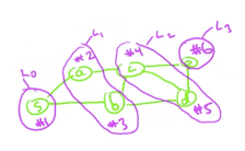
The algorithm systematically explores the nodes in "layers", using a cautious and tentative approach. The starting node will be in its own layer. The neighbors of s will constitute layer 1, and so on. There is a close correspondence between these layers and shortest path distances. The algorithm is implemented using a queue (FIFO).

The algorithm is linear time O(n + m) with small constants.

BFS can be used to:

• compute shortest paths
• compute connected components of an undirected graph

BFS Algorithm Pseudocode

The general idea is to start from a node, mark it as explored and put it in a queue. Then, in a while loop as long as the queue has elements, remove the head of the queue, which is always explored, determine its adjacent unexplored nodes - in the same layer, mark them as explored and put them at the back of the queue. Ignore the adjacent explored node, to avoid doing unnecessary work The queue always contains explored nodes at the frontier between the explored area and the unexplored area. Iterate until the queue is empty and the whole connected component is explored.

BFS works with both undirected and directed graphs.

BFS(graph G, start vertex s)
  # All nodes are assumed unexplored
  initialize a Queue Q (FIFO)
  mark s as explored
  place s in Q
  while Q has elements
    remove the head of the queue v
    for each edge (v, w):
      if w unexplored:
        mark w as explored
        add w to Q

When we "mark as explored" we can actually annotate each node marked as explored with a value of a distance from s that indicates the layers the nodes are in. This is how to count shortest path in graphs.

BFS Running Time

The runtime analysis of the algorithm described above follows. The running time of the main loop, ignoring any kind of pre-processing or initialization, is proportional to the number of nodes that can be reached from s and the number of edges that can be reached from s: O(n_s + m_s). The total work done in the while loop, we will only deal with the vertices findable from s (n_s). For each given node we insert it from the queue and we remove it from the queue, which is constant work. We will never deal with a single node more than once. For a given edge we might look at it twice. For an edge (v, w) we may consider it once when we look at the vertex v and we might consider it again when we look at the vertex w. Each time we look at an edge we do constant work. The overall over time is going to be proportional to the number of vertices findable from s and number of edges findable from s.

BFS Applications

Find the Shortest Path in a Graph

Shortest Path in a Graph

Find Connected Components in an Undirected Graphs

Find Connected Components in an Undirected Graph

Depth-First Search (DFS)

https://www.coursera.org/learn/algorithms-graphs-data-structures/lecture/pKr0Y/depth-first-search-dfs-the-basics

External: CLRS page 603.

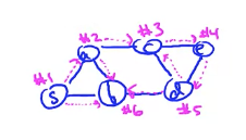
Depth-first search performs a more aggressive search than BFS. It explores the graph as deep as it can while backtracking only when necessary. It uses a different data structure, a stack (LIFO). A practical implementation of the algorithm uses recurrence instead of an explicit stack: the stack structure is implicitly implemented by the recursive calls. The algorithm is linear time O(n + m) with small constants.

DFS Iterative Algorithm Pseudocode

The general idea is to start from a node, mark it as explored and put it at the top of a stack (LIFO). Then, in a while loop as long as the stack has elements, pop the top of the stack, which is always explored, determine its adjacent unexplored nodes, choose one, mark it as explored and put it at the top of the stack. Ignore the adjacent explored node, to avoid doing unnecessary work The stack always contains explored nodes at the frontier between the explored area and the unexplored area. Iterate until the stack is empty and the whole connected component is explored. The "aggressiveness" of the algorithm comes from the fact that it chooses an unexplored node that is farther and farther away from the start node, aways biased towards the most recently discovered explored nodes, and backtracks when it runs out of options, as opposite to BFS that favors nodes arranged in layers at the same distance from the start node.

Iterative_DFS(graph G, start vertex s)
  # All nodes are assumed unexplored
  initialize a Stack S (LIFO)
  mark s as explored
  push s at the top of S
  while S has elements
    pop the top of the stack v
    for each edge (v, w):
      if w unexplored:
        mark w as explored
        push w at the top of S

DFS Recursive Algorithm Pseudocode

The explicit use of a stack can be naturally replaced with a recursive call:

Recursive_DFS(graph G, start vertex s)
  mark s as explored
  for every edge (s, v):
    if v unexplored:
      Recursive_DFS(G, v)

DFS Applications

Topological Sort of a Directed Acyclic Graph

Topological Sort of a Directed Acyclic Graph

Find Strongly Connected Components of a Directed Graph

Find Strongly Connected Components in a Directed Graph (Kosaraju's Algorithm)