Dijkstra's Shortest-Path Algorithm

External

• https://www.coursera.org/learn/algorithms-graphs-data-structures/lecture/rxrPa/dijkstras-shortest-path-algorithm
• https://www.coursera.org/learn/algorithms-graphs-data-structures/lecture/iIzo8/heaps-operations-and-applications
• https://www.coursera.org/learn/algorithms-graphs-data-structures/lecture/Jfvmn/dijkstras-algorithm-examples
• https://www.coursera.org/learn/algorithms-graphs-data-structures/lecture/VCHYw/correctness-of-dijkstras-algorithm
• https://www.coursera.org/learn/algorithms-graphs-data-structures/lecture/Pbpp9/dijkstras-algorithm-implementation-and-running-time

Internal

• Shortest Path in a Graph

Overview

The problem of computing the shortest path in a graph can be solved with bread-first search, but the breadth-first search-based shortest path algorithm works in the special case when the length of every edge in the graph ℓe is 1. Dijkstra's shortest-path algorithm solves a more general problem, where the edges have arbitrary non-negative lengths.

The problem of computing the shortest path in a graph with arbitrary edge lengths can be theoretically reduced to the problem of computing the shortest path in a graph with edges of length ℓe=1, by replacing an edge with an arbitrary length n with n edges with length 1, and adding extra vertices. The breadth-first search-based shortest path algorithm would theoretically work fine in this situation, producing the same results as the Dijkstra's algorithm, but the problem is that we are increasing the size of the graph, in terms of adding extra nodes and edges, and this increase my be non-trivial: for an edge with length 1000, we need to add extra 999 edges and 999 extra nodes. This representation would be wasteful, and even if the breadth-first search-based shortest path algorithm works in linear time, it is on a much larger graph, and we would much prefer an linear-time (or close to linear-time algorithm) that achieves the same result on the smaller graph. This is exactly what the Dijkstra's algorithm accomplishes.

If all edges are unit-length edges, Dijkstra's becomes the breadth-first search-based algorithm.

The Problem

The single-source shortest paths is formally defined as follows: given a directed graph G=(V, E) , with n = │V│ and m=│E│, where each edge e has a non-negative length ℓ_e, and a source vertex s, compute for each v ∈ V the length L(v) of the shortest path s → v.

The assumption that the length is non-negative is important. Dijkstra's shortest-path algorithm does not work correctly in presence of negative length edges.

Directed vs. Undirected Graphs

The Dijkstra's algorithm is defined below for directed graphs, but works with minimal modifications on undirected graphs. The difference consists in considering all edges that cross the boundary between the explored and unexplored territory, instead of just the directed edges, in the algorithm described below.

The Non-Optimized Implementation

The general idea is to start at the source vertex s, and iterate in such a way that in each iteration we explore a new vertex and add it to the "explored territory".

The new vertex is chosen in such a way that it minimizes Dijkstra's Greedy Criterion, as described below.

 Initialize X={s} # X is the set of vertices for which the shortest path to s has been computed so far
 Initialize A[s]={0} # A maintains computed shortest path distances from the vertices explored so far to s
 Initialize B[s]={empty path} # B maintains the actual shortest path distances from the vertices explored 
                              # so far to s. This is not necessary in the algorithm but helps with the 
                              # understanding of the algorithm.

 while X ≠ V: # The main loop, each iteration grows X with one node
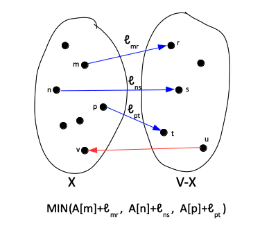
     for every directed edge (v, w) ∈ E that crosses X/(V-X) boundary v ∈ V, w ∈ V-X
         pick the (v*, w*) edge that minimizes A[v] + ℓvw # The Dijkstra's Greedy Criterion
     add w* to X
     set A[w*] = A[v*] + ℓv*w*
     set B[w*] = B[v*] ⋃ (v*,w*)

Dijkstra's Greedy Criterion

At each step, for every directed edge (v, w) ∈ E that crosses X/(V-X) boundary v ∈ V, w ∈ V-X, minimize:

A[v] + ℓvw

and pick the edge that has the minimal value for this criterion. The expression A[v]+ℓ_vw is known as Dijkstra's greedy score.

Examples

https://www.coursera.org/learn/algorithms-graphs-data-structures/lecture/Jfvmn/dijkstras-algorithm-examples

Playground Implementation

https://github.com/ovidiuf/playground/blob/master/learning/stanford-algorithms-specialization/07-dijkstra-shortest-path/src/main/java/playground/stanford/dijkstra/NonOptimizedDijkstra.java

Negative Edge Length Intuition

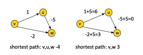
One approach would be to try to reduce the problem of computing shortest path with negative edge length to the problem of computing the shortest path with non-negative edge lengths, by adding a big number to all the edges that makes them all non-negative. The problem with this approach is that different paths between a source and destination vertex have different number of edges, and adding the same amount to each edge in the graph affects different paths in different ways - change path lengths by different amounts, so this reduction does not work. The reduction does not preserve the shortest path. This is immediately noticeable in the following example:

Another intuition is that Dijkstra's algorithm commits to the shortest path identified so far as being the shortest. If there are negative edges, this has the potential to reduce the length, in the future. This idea can be formally used in the inductive proof.

Correctness

https://www.coursera.org/learn/algorithms-graphs-data-structures/lecture/VCHYw/correctness-of-dijkstras-algorithm

The Optimized Implementation

https://www.coursera.org/learn/algorithms-graphs-data-structures/lecture/Pbpp9/dijkstras-algorithm-implementation-and-running-time

In the non-optimized version of the algorithm, there was a step, repeated for each remaining graph vertex, where we needed to consider all edges traversing the boundary between explored and non-explored territory, and find out a minimum of the Dijkstra's Greedy Criterion. The number of edges is O(m) so the non-optimized version of the algorithm has a O(n*m) running time.

The optimization comes from the idea to use a use of a heap when choosing what edge to pick. We use the heap to actually store vertices, not edges. All nodes in V - X will be maintained in a heap structure. Because we're storing vertices rather than edges, special care should be taken with how we are going to define the keys in the heap. We are going to maintain the property that the key of a vertex v in V-X key[v] is the smallest Dijkstra greedy score of any edge that has that vertex as its head.

The one step from the unoptimized algorithm - examining all edges that cross the boundary in a linear search to find the one with the smallest greedy score - turns into a two steps process. The first step is local: each vertex in the unexamined territory looks at its edges and determines the one with the minimum Dijkstra score. This score becomes the heap key of the vertex. In the second step is global: the vertex with the minimal key is identified via the heap - it sits at the top of the heap. The key, and the corresponding vertex is extracted with REMOVE-MIN(). The heap is going to return to us in O(log n) the same vertex that in the unoptimized version of the algorithm was returned as a result of an O(m) exhaustive search.

At this stage, the Dijkstra greedy score is provided as the value of the key and can be used as the length of the path:

A[w*] = key[w*]

After processing the current vertex, it is moved from outside X to inside X. The frontier between X and V-X changes, so the edges that cross the frontier change. Edges that used to not cross the frontier may cross the frontier. For vertices that remain in the heap, the greedy score might have dropped. The vertices whose keys we need to update are precisely those that are the head of edges whose tail is the node just processed. The way we update the key is to remove the vertex from the heap, compute the key, and re-insert it in the heap:

When w extracted from the heap (added to X)
  if v ∈ V-X (in the heap)
    delete v from the heap
    recompute key[v] = min(key[v], A[w] + ℓwv)
    re-insert v into the heap

The optimized algorithm running time is O(n log n).